8 Manipulando rasters

Vamos utilizar os dados volcano presentes no software R, o qual possui informações topográficas (elevação) do vulcão Maunga Whau de Auckland na Nova Zelândia.

8.1 Dados de altitude de um vulcão

Vamos carregar os pacotes necessários:

library(raster)
library(RColorBrewer)
library(sf)
library(tmap)
library(tidyverse)
library(rnaturalearth)

volcano[1:5, 1:5]

     [,1] [,2] [,3] [,4] [,5]
[1,]  100  100  101  101  101
[2,]  101  101  102  102  102
[3,]  102  102  103  103  103
[4,]  103  103  104  104  104
[5,]  104  104  105  105  105

Vamos transformar essa matriz de dados em um raster.

raster_layer <- raster(volcano)
raster_layer

class      : RasterLayer 
dimensions : 87, 61, 5307  (nrow, ncol, ncell)
resolution : 0.01639344, 0.01149425  (x, y)
extent     : 0, 1, 0, 1  (xmin, xmax, ymin, ymax)
crs        : NA 
source     : memory
names      : layer 
values     : 94, 195  (min, max)

plot(raster_layer, col = viridis::viridis(8))

Agora, vamos criar um raster brick a partir de vários raster layers.

# Raster layers
raster_layer1 <- raster_layer
raster_layer2 <- raster_layer * raster_layer
raster_layer3 <- sqrt(raster_layer)
raster_layer4 <- log10(raster_layer)

# Raster brick
raster_brick <- brick(raster_layer1, raster_layer2, raster_layer3, raster_layer4)
raster_brick

class      : RasterBrick 
dimensions : 87, 61, 5307, 4  (nrow, ncol, ncell, nlayers)
resolution : 0.01639344, 0.01149425  (x, y)
extent     : 0, 1, 0, 1  (xmin, xmax, ymin, ymax)
crs        : NA 
source     : memory
names      :      layer.1,      layer.2,      layer.3,      layer.4 
min values :    94.000000,  8836.000000,     9.695360,     1.973128 
max values :   195.000000, 38025.000000,    13.964240,     2.290035

plot(raster_brick, col = viridis::viridis(8))

9 RasterLayer

9.1 Umidade do solo

Faça o download do arquivo “SMAP_SM.tif” em: https://github.com/Vinit-Sehgal/SampleData/tree/master/raster_files

sm=raster("SMAP_SM.tif")
print(sm)

class      : RasterLayer 
dimensions : 456, 964, 439584  (nrow, ncol, ncell)
resolution : 0.373444, 0.373444  (x, y)
extent     : -180, 180, -85.24595, 85.0445  (xmin, xmax, ymin, ymax)
crs        : +proj=longlat +datum=WGS84 +no_defs 
source     : SMAP_SM.tif 
names      : SMAP_SM 
values     : 0.01999998, 0.8766761  (min, max)

plot(sm, main="Umidade do solo")

plot(sm, main="Umidade do solo",
col=brewer.pal(10,"Spectral"),
lab.breaks=seq(0, 1, by=0.1),
breaks=seq(0, 1, by=0.1),
colNA="lightgray",
axes=TRUE,
lim=c(-180, 180),
ylim=c(-90, 90),
zlim=c(0,1),
xlab="Longitude",
ylab="Latitue",)

9.2 Dados climáticos

Download de dados climáticos: Acesse: https://www.worldclim.org/data/worldclim21.html Baixe os dados bioclimáticos históricos com resolução de 2.5 minutos (BIOCLIM 2.5m).

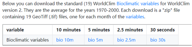
Ao descompactar os dados climáticos do WorldClim, você encontrará várias variáveis bioclimáticas disponíveis.

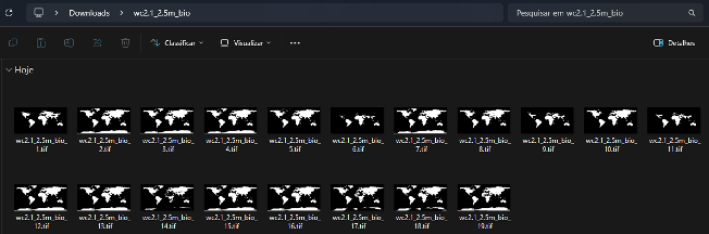
Cada arquivo corresponde a uma variável climática específica, com resolução espacial de 2.5 minutos. Elas são a média para os anos de 1970-2000. BIO1 = Temperatura média anual BIO2 = Amplitude média diária BIO3 = Isotermalidade (BIO2/BIO7) (×100) BIO4 = Sazonalidade da temperatura (desvio padrão ×100) BIO5 = Temperatura Máxima do Mês Mais Quente BIO6 = Temperatura mínima do mês mais frio BIO7 = Amplitude anual de temperatura (BIO5-BIO6) BIO8 = Temperatura média do trimestre mais chuvoso BIO9 = Temperatura média do trimestre mais seco BIO10 = Temperatura média do trimestre mais quente BIO11 = Temperatura média do trimestre mais frio BIO12 = Precipitação Anual BIO13 = Precipitação do mês mais chuvoso BIO14 = Precipitação do mês mais seco BIO15 = Sazonalidade da Precipitação (Coeficiente de Variação) BIO16 = Precipitação do trimestre mais chuvoso BIO17 = Precipitação do trimestre mais seco BIO18 = Precipitação do trimestre mais quente BIO19 = Precipitação do trimestre mais frio

9.2.1 Precipitação anual

# Carregar o raster bio12
climate_bio12 <- raster("wc2.1_2.5m_bio/wc2.1_2.5m_bio_12.tif")
extent(climate_bio12)

class      : Extent 
xmin       : -180 
xmax       : 180 
ymin       : -90 
ymax       : 90

# Mapa básico
tm_shape(climate_bio12) +
tm_raster() +
tm_layout(legend.position = c("left", "bottom"))

cores_rcolorbrewer <- brewer.pal(5, "Set2")

# Mapa final 
tm_shape(climate_bio12) + 
  tm_raster(palette = cores_rcolorbrewer, breaks = c(0, 2000, 4000, 6000, 8000, 10000, 12000), labels = c("0 até 2000", "2001 até 4000", "4001 até 6000", "6001 até 8000","8001 até 10000", "10001 até 12000"), title = "Precipitação anual (mm/yr)") + 
  tm_layout(main.title = "Média de Precipitação Anual Mundial", main.title.position = "center",legend.position = c("left", "bottom")) + 
  tmap_save(filename = "map_prec_mun.png", width = 20, height = 20, units = "cm", dpi = 600)

9.2.1.1 África

# Baixar dados de países da África
africa <- ne_countries(continent = 'africa', returnclass = 'sf')

# Obter a extensão da África
africa_extent <- st_bbox(africa)
africa_extent

     xmin      ymin      xmax      ymax 
-17.62504 -34.81917  51.13387  37.34999

# Recortar os dados climáticos para a área da África usando a extensão obtida
climate_africa <- crop(climate_bio12, extent(africa_extent$xmin, africa_extent$xmax, africa_extent$ymin, africa_extent$ymax))
climate_africa

class      : RasterLayer 
dimensions : 1732, 1650, 2857800  (nrow, ncol, ncell)
resolution : 0.04166667, 0.04166667  (x, y)
extent     : -17.625, 51.125, -34.83333, 37.33333  (xmin, xmax, ymin, ymax)
crs        : +proj=longlat +datum=WGS84 +no_defs 
source     : memory
names      : wc2.1_2.5m_bio_12 
values     : 0, 4526  (min, max)

# Convertendo o raster para um data frame e removendo valores NA
rasdf <- as.data.frame(climate_africa, xy = TRUE) %>% drop_na()

# Plotagem com ggplot2
ggplot() +
geom_raster(aes(x = x, y = y, fill = wc2.1_2.5m_bio_12), data = rasdf) +
geom_sf(fill = 'transparent', data = africa) +
scale_fill_viridis_c(name = 'mm/yr', direction = -1) +
labs(x = 'Longitude', y = 'Latitude',
title = "Mapa climático da África", subtitle = 'Precipitação anual')

9.2.1.2 Brasil

# Baixar dados de países do Brasil
brazil <- ne_countries(country = 'Brazil', returnclass = 'sf')

# Obter a extensão do Brasil
brazil_extent <- st_bbox(brazil)

# Recortar os dados climáticos para a área do Brasil usando a extensão obtida
climate_brazil <- crop(climate_bio12, extent(brazil_extent$xmin, brazil_extent$xmax, brazil_extent$ymin, brazil_extent$ymax))

# Convertendo o raster para um data frame e removendo valores NA
rasdf <- as.data.frame(climate_brazil, xy = TRUE) %>% drop_na()

# Plotagem com ggplot2
ggplot() +
  geom_raster(aes(x = x, y = y, fill = wc2.1_2.5m_bio_12), data = rasdf) +
  geom_sf(fill = 'transparent', data = brazil) +
  scale_fill_viridis_c(name = 'mm/yr', direction = -1) +
  labs(x = 'Longitude', y = 'Latitude',
  title = "Mapa climático do Brasil", subtitle = 'Precipitação anual')

9.2.2 Temperatura média anual

# Carregar o raster bio1
climate_bio1 <- raster("wc2.1_2.5m_bio/wc2.1_2.5m_bio_1.tif")
extent(climate_bio1)

class      : Extent 
xmin       : -180 
xmax       : 180 
ymin       : -90 
ymax       : 90

# Mapa básico
tm_shape(climate_bio1) +
tm_raster() +
tm_layout(legend.position = c("left", "bottom"))

# Mapa final 
tm_shape(climate_bio1) + 
  tm_raster(palette = "Blues", breaks = c(-60, -40, -20, 0, 20, 40), labels = c("-60 até -40", "-39 até -20", "-19 até 0", "1 até 20","20 até 40"), title = "ºC") +
  tm_layout(main.title = "Média da Temperatura Anual Mundial", main.title.position = "center",legend.position = c("left", "bottom")) + 
  tmap_save(filename = "map_temp_mun.png", width = 20, height = 20, units = "cm", dpi = 600)

9.2.2.1 África

# Recortar os dados climáticos para a área da África usando a extensão obtida
climate_africa <- crop(climate_bio1, extent(africa_extent$xmin, africa_extent$xmax, africa_extent$ymin, africa_extent$ymax))

# Recortar os dados climáticos para a área da África usando a extensão obtida
climate_africa <- crop(climate_bio1, extent(africa_extent$xmin, africa_extent$xmax, africa_extent$ymin, africa_extent$ymax))

# Plotagem com ggplot2
ggplot() +
  geom_raster(aes(x = x, y = y, fill = wc2.1_2.5m_bio_12), data = rasdf) +
  geom_sf(fill = 'transparent', data = africa) + 
  scale_fill_viridis_c(name = '°C', direction = -1) +
  labs(x = 'Longitude', y = 'Latitude', title = "Mapa de Temperatura Média Anual da África")

9.2.2.2 Brasil

# Recortar os dados climáticos para a área do Brasil usando a extensão obtida
climate_brazil <- crop(climate_bio1, extent(brazil_extent$xmin, brazil_extent$xmax, brazil_extent$ymin, brazil_extent$ymax))

# Convertendo o raster para um data frame e removendo valores NA
rasdf <- as.data.frame(climate_brazil, xy = TRUE) %>% drop_na()

# Plotagem com ggplot2
ggplot() +
  geom_raster(aes(x = x, y = y, fill = wc2.1_2.5m_bio_1), data = rasdf) +
  geom_sf(fill = 'transparent', data = brazil) +
  scale_fill_viridis_c(name = '°C', direction = -1) +
  labs(x = 'Longitude', y = 'Latitude', title = "Mapa de Temperatura Média Anual do Brasil")